NetCDF data and R
Keywords: data format, NetCDF, R,
Apologies for the extreme hiatus in blog posts. I am going to ease back into things by discussing NetCDF files and how to work with them in R. In recent years, NetCDF files have gained popularity especially for climatology, meteorology, remote sensing, oceanographic and GIS data applications. As you would have guessed it, NetCDF is an acronym that stands for Network Common Data Form. NetCDF and can be described as an open-source array-oriented data storage format.
Here are a few examples of data stored in NetCDF format:
Climate data from https://climate.copernicus.eu/.
Climate and atmospheric data from https://www.ecmwf.int/.
Climate data from https://climatedataguide.ucar.edu/.
Oceanographic data from NOAA.
Antarctic bathymetry data. Here is a blog post on rOpenSci.org discussing retrieval of Antarctic bathymetry data.
Everglades Water level data from US Geological Survey.
For this blog post I will walk through my exploration of working with NetCDF files in R using the Everglades water level data (above) as an example. The data is actually a double whammy, its geospatial and hydrologic data. This blog post is ultimately bits and pieces of other blog posts scatter around the web. I hope you find it useful.
First lets load the necessary R-packages/libraries.
# Libraries
library(chron) # package for creating chronological objects
library(ncdf4)  # package to handle NetCDF

library(raster) # package for raster manipulation
library(rgdal) # package for geospatial analysis
library(tmap) # package for plotting map data
library(RColorBrewer) # package for color palettes
Navigate to the data website and pick a data file. I decided on 2017_Q4 (link will download a file). Once the file is downloaded, unzip the file using either R with the unzip() function or some other decompression software/operating system tools.
Alright now that the file is downloaded and unzipped lets open the file. I created an variable called working.dir which is a string indicating my “working directory” location (working.dir<-"D:/UF/_Working_Blog/NetCDFBlog") and points me to where I downloaded and unzipped the data file.
Excellent! The data is now in the R-environment, let take a look at the data.
## File D:/UF/_Working_Blog/NetCDFBlog/USGS_EDEN/2017_q4.nc (NC_FORMAT_CLASSIC):
##
##      2 variables (excluding dimension variables):
##         float stage[x,y,time]
##             long_name: stage
##             esri_pe_string: PROJCS["NAD_1983_UTM_Zone_17N",GEOGCS["GCS_North_American_1983",DATUM["D_North_American_1983",SPHEROID["GRS_1980",6378137.0,298.257222101]],PRIMEM["Greenwich",0.0],UNIT["Degree",0.0174532925199433]],PROJECTION["Transverse_Mercator"],PARAMETER["False_Easting",500000.0],PARAMETER["False_Northing",0.0],PARAMETER["Central_Meridian",-81.0],PARAMETER["Scale_Factor",0.9996],PARAMETER["Latitude_Of_Origin",0.0],UNIT["Meter",1.0]]
##             coordinates: x y
##             grid_mapping: transverse_mercator
##             units: cm
##             min: -8.33670043945312
##             max: 499.500701904297
##         int transverse_mercator[]
##             grid_mapping_name: transverse_mercator
##             longitude_of_central_meridian: -81
##             latitude_of_projection_origin: 0
##             scale_factor_at_central_meridian: 0.9996
##             false_easting: 5e+05
##             false_northing: 0
##             semi_major_axis: 6378137
##             inverse_flattening: 298.257222101
##
##      3 dimensions:
##         time  Size:92
##             long_name: model timestep
##             units: days since 2017-10-01T12:00:00Z
##         y  Size:405
##             long_name: y coordinate of projection
##             standard_name: projection_y_coordinate
##             units: m
##         x  Size:287
##             long_name: x coordinate of projection
##             standard_name: projection_x_coordinate
##             units: m
##
##     2 global attributes:
##         Conventions: CF-1.0
##         Source_Software: JEM NetCDF writer
As you can see all the metadata needed to understand what the dat.nc file is lives in the file. Definately a pro for using NetCDF files. Now lets extract our three dimensions (latitude, longitude and time).
lon <- ncvar_get(dat.nc,"x");# extracts longitude
nlon <- dim(lon);# returns the number of records

lat <- ncvar_get(dat.nc,"y");# extracts latitude
nlat <- dim(lat);# returns the number of records

time <- ncvar_get(dat.nc,"time");# extracts time
tunits <- ncatt_get(dat.nc,"time","units");# assigns units to time
nt <- dim(time)
Now that we have our coordinates in space and time extracted let get to the actual data. If you remember when we viewed the dataset using print() sifting through the output you’ll notice long_name: stage, that is our data.
dname="stage"
tmp_array <- ncvar_get(dat.nc,dname)
dlname <- ncatt_get(dat.nc,dname,"long_name")
dunits <- ncatt_get(dat.nc,dname,"units")
fillvalue <- ncatt_get(dat.nc,dname,"_FillValue")
We can also extract other information including global attributes such as title, source, references, etc. from the datasets metadata.
# get global attributes
title <- ncatt_get(dat.nc,0,"title")
institution <- ncatt_get(dat.nc,0,"institution")
datasource <- ncatt_get(dat.nc,0,"source")
references <- ncatt_get(dat.nc,0,"references")
history <- ncatt_get(dat.nc,0,"history")
Conventions <- ncatt_get(dat.nc,0,"Conventions")
Now that we got everything we wanted from the NetCDF file we can “close” the connection by using nc_close(dat.nc).
The data we just extracted from this NetCDF file is a time-series of daily spatially interpolated water level data across a large ecosystem (several thousand km2). Using the chron library lets format this data to something more workable by extracting the date information from tunits$value and time variables.
tustr <- strsplit(tunits$value, " ")
tdstr <- strsplit(unlist(tustr)[3], "-")
tmonth <- as.integer(unlist(tdstr)[2])
tday <- as.integer(substring(unlist(tdstr)[3],1,2))
tyear <- as.integer(unlist(tdstr)[1])
time.val=as.Date(chron(time,origin=c(tmonth, tday, tyear)))
We know from both the metadata information within the file and information from where we retrieved the data that this NetCDF is an array representing the fourth quarter of 2017. This information combined with the extracted day, month and year information above we can determine the date corresponding to each file within the NetCDF array
## [1] "2017-10-01" "2017-10-02" "2017-10-03" "2017-10-04" "2017-10-05"
## [6] "2017-10-06"
Like most data, sometime values of a variable are missing or not available (outside of modeling domain) and are identified using a specific “fill value” (_FillValue) or “missing value” (missing_value). To replace theses values its pretty simple and similar to that of a normal data frame.
To count the number of data points (i.e. non-NA values) you can use length(na.omit(as.vector(tmp_array[,,1])))
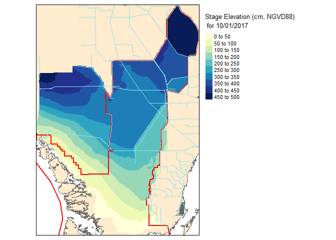
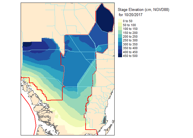
Now that the data is extracted, sorted and cleaned lets take a couple of slices from this beautiful NetDF pie.
## [1] "2017-10-01"## [1] "2017-10-20"Before we get to the mapping nitty gritty visit my prior blog post on Mapping in #rstats. To generate the maps I will be using the tmap library.
If you notice the slice1 and slice2 are “Large matrix” files and not spatial files yet. Remember back when we looked at the metadata in the file header using print(dat.nc)? It identified the spatial projection of the data in the esri_pe_string: field. During the process of extracting the NetCDF slice and the associated transformation to a raster the data is i the wrong orientation therefore we have to use the flip() function to get it pointed in the correct direction.
#Defining the projection
utm17.pro=CRS("+proj=utm +zone=17 +ellps=GRS80 +towgs84=0,0,0,0,0,0,0 +units=m +no_defs")

slice1.r <- raster(t(slice1), xmn=min(lon), xmx=max(lon), ymn=min(lat), ymx=max(lat),crs=utm17.pro)
slice1.r <- flip(slice1.r, direction='y')

slice2.r <- raster(t(slice2), xmn=min(lon), xmx=max(lon), ymn=min(lat), ymx=max(lat),crs=utm17.pro)
slice2.r <- flip(slice2.r, direction='y')
Now lets take a look at our work!
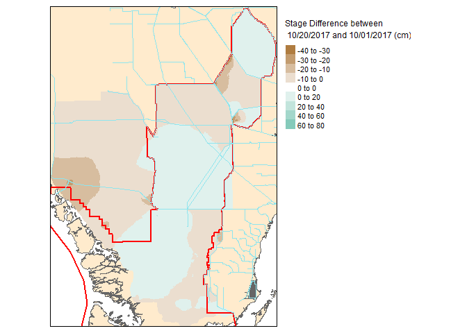
Now that these slices are raster files, you can take it one step further and do raster based maths…for instance seeing the change in water level between the two dates.