Upper Tolerance interval for censored data

Computes a one-sided upper tolerance interval for censored data assuming log-normal, gamma and normal distributions.

cenTolInt(
  x.var,
  cens.var,
  conf = 0.95,
  cover = 0.9,
  method.fit = "mle",
  printstat = TRUE
)

Arguments

x.var: The column of x (response variable) values plus detection limits
cens.var: The column of indicators, where 1 (or TRUE) indicates a detection limit in the y.var column, and 0 (or FALSE) indicates a detected value in y.var.
conf: Confidence coefficient of the interval, 0.95 (default).
cover: Coverage, the percentile probability above which the tolerance interval is computed. The default is 90, so a tolerance interval will be computed above the 90th percentile of the data.
method.fit: The method used to compute the parameters of the distribution. The default is maximum likelihood (“mle”). The alternative is robust ROS (“rROS”). See Details.
printstat: Logical TRUE/FALSE option of whether to print the resulting statistics in the console window, or not. Default is TRUE.

Value

Prints and returns the percentile (cover), upper tolerance limit (conf) and BIC of fit for lognormal, normal and approximated gamma distributions. Plots empirical and theoretical CDFs with BIC values in the legend.

Details

Computes upper one-sided tolerance intervals for three distributions. This is a front-end to the individual functions from the EnvStats package. By default all three are computed using maximum likelihood estimation (mle); robust ROS is available as an alternate method for all three distributions. The gamma distribution for censored data uses the Wilson-Hilferty approximation (normal distribution on cube roots of data). For more info on the relative merits of robust ROS versus mle, see Helsel (2011) and Millard (2013).

References

Helsel, D.R., 2011. Statistics for censored environmental data using Minitab and R, 2nd ed. John Wiley & Sons, USA, N.J.

Millard, S.P., 2013. EnvStats: An R Package for Environmental Statistics. Springer-Verlag, New York.

Krishnamoorthy, K., Mathew, T., Mukherjee, S., 2008. Normal-Based Methods for a Gamma Distribution, Technometrics, 50, 69-78.

Examples


data(PbHeron)

# Default
cenTolInt(PbHeron$Liver,PbHeron$LiverCen)
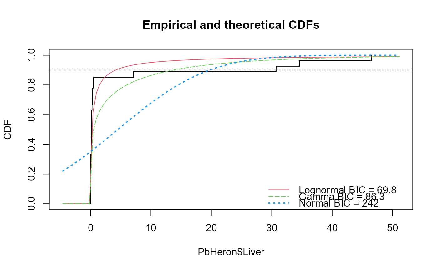#>   Distribution 90th Pctl  95% UTL       BIC Method
#> 1    Lognormal  4.156275 14.48148  69.80314    mle
#> 2        Gamma  9.080911 18.22023  86.31145    mle
#> 3       Normal 19.957630 26.91080 242.48001    mle

# User defined conficence interval
cenTolInt(PbHeron$Liver,PbHeron$LiverCen,conf=0.75)

#>   Distribution 90th Pctl   75% UTL       BIC Method
#> 1    Lognormal  4.156275  6.743991  69.80314    mle
#> 2        Gamma  9.080911 12.130005  86.31145    mle
#> 3       Normal 19.957630 22.653852 242.48001    mle

# User defined percentile
cenTolInt(PbHeron$Liver,PbHeron$LiverCen,cover=0.5)

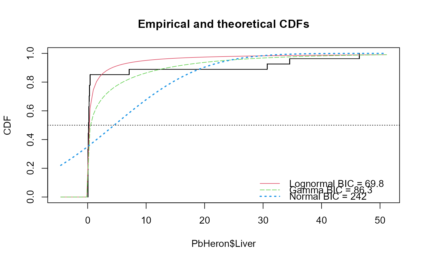#>   Distribution 50th Pctl   95% UTL       BIC Method
#> 1    Lognormal 0.2029654 0.4398284  69.80314    mle
#> 2        Gamma 0.4526509 1.3511311  86.31145    mle
#> 3       Normal 3.1389176 7.4467275 242.48001    mle

# inputs outside acceptable ranges
# Will result in errors/warnings
# cenTolInt(PbHeron$Liver,PbHeron$LiverCen,cover=1.25)
# cenTolInt(PbHeron$Liver,PbHeron$LiverCen,conf=1.1)
# cenTolInt(PbHeron$Liver,PbHeron$LiverCen,method.fit="ROS")