
Nearest Neighbor and Hot Spot Analysis - Geospatial data analysis in #rstats. Part 3b
Keywords: geostatistics, R, nearest neighbor, Getis-Ord
As promised here is another follow-up to our Geospatial data analysis blog series. So far we have covered interpolaiton, spatial auto-correlation and the basics of Hot-Spot (Getis-Ord) analysis.
Part I: Interpolation
Part 2: Spatial Autocorrelation
Part 3: Hot Spot Analysis
In this post we will discuss nearest neighbor estimates and how it can affect hot spot detection. In essence this is “Getis-Ord Strikes Back” (sorry my Star Wars nerd is showing).
Let’s take a step back before jumping back into nearest neighbor (see my post on Moran’s I). Most spatial statistics compare a test statistic estimated from the data then compared to an expected value given the null hypothesis of complete spatial randomness (CSR; Fortin and Dale (2005); not to be confused with CRS(...) coordinate reference system). This is a point process model that can be estimated from a particular distribution, in most cases a Poisson (Diggle 2006). A theme in the analysis of spatial point patterns such as Moran’s I, Getis-Ord G or Ripley’s K provides a distinction between spatial patterns where CSR is a dividing hypothesis (Cox 1977), which leads to classification of random (complete spatial randomness), under-dispersed (clumped or aggregated), or over-dispersed (spaced or regular) patterns.
Below we are going to import some data, use different techniques to estimate nearest neighbor and see how that affects Hot spot detection.
Let’s get started
Before we get too deep into things here are the necessary packages we will be using.
## Libraries
# read xlsx files
library(readxl)

# Geospatial
library(rgdal)
library(rgeos)
library(raster)
library(spdep)
Same data and links from last post.
# Define spatial datum
utm17<-CRS("+proj=utm +zone=17 +datum=WGS84 +units=m")
wgs84<-CRS("+proj=longlat +datum=WGS84 +no_defs +ellps=WGS84 +towgs84=0,0,0")

# Read shapefile
wcas<-readOGR(GISdata,"WCAs")
wcas<-spTransform(wcas,utm17)

# Read the spreadsheet
p12<-readxl::read_xls("data/P12join7FINAL.xls",sheet=2)

# Clean up the headers
colnames(p12)<-sapply(strsplit(names(p12),"\\$"),"[",1)
p12<-data.frame(p12)
p12[p12==-9999]<-NA
p12[p12==-3047.6952]<-NA

# Convert the data.frame() to SpatialPointsDataFrame
vars<-c("STA_ID","CYCLE","SUBAREA","DECLONG","DECLAT","DATE","TPSDF")
p12.shp<-SpatialPointsDataFrame(coords=p12[,c("DECLONG","DECLAT")],
                               data=p12[,vars],proj4string =wgs84)
# transform to UTM (something I like to do...but not necessary)
p12.shp<-spTransform(p12.shp,utm17)

# Subset the data for wet season data only and only WCA sites
p12.shp2<-subset(p12.shp,CYCLE%in%c(0,2))
p12.shp.wca<-p12.shp2[wcas,]

# Double check for NAs in the dataset
subset(p12.shp.wca@data,is.na(TPSDF)==T)

# Remove NA sample
p12.shp.wca<-subset(p12.shp.wca,is.na(TPSDF)==F)
Here is a quick map the of the subsetted data
par(mar=c(0.1,0.1,0.1,0.1),oma=c(0,0,0,0))
plot(wcas)
plot(p12.shp.wca,pch=21,bg=adjustcolor("dodgerblue1",0.5),cex=1,add=T)
mapmisc::scaleBar(utm17,"bottomright",bty="n",cex=1,seg.len=4)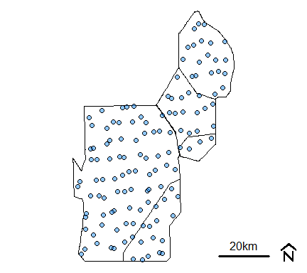
Monitoring location from R-EMAP Phase I, wet season sampling (cycles 0 and 2) within the Water Conservation Areas.
Nearest Neighbor
As discussed in our prior blog post, average nearest neighbor (ANN) analysis measures the average distance from each point in the study area to its nearest point. In some cases, this methods can be sensitive to which distance bands are identified and can therefore be carried forward into other analyses that rely on nearest neighbor spatial weighting. However, ANN statistic is one of many distance based point pattern analysis statistics that can be used to spatially weight the dataset necessary for spatial statistical evaluation. Others include K, L and pair correlation function (g; not to confused with Getis-Ord G) (Gimond 2020).
One way to spatially weight the data is by using the dnearneigh() function which identifies neighbors within the lower and upper bounds (provided in the function) by Euclidean distance. Here is where selection of “distance bands” matter. This function was used in the initial Hot-Spot blog post. Lets see how changing the upper bounds in the dnearneigh() can affect the outcome.
# Find distance range
ptdist=pointDistance(p12.shp.wca)

min.dist<-min(ptdist); # Minimum

q10.dist<-as.numeric(quantile(ptdist,probs=0.10)); # Q10
q25.dist<-as.numeric(quantile(ptdist,probs=0.25)); # Q25
q75.dist<-as.numeric(quantile(ptdist,probs=0.75)); # Q75

# Using 25th percentile distance for upper bound
nb.q10<-dnearneigh(coordinates(p12.shp.wca),min.dist,q10.dist)

# Using 25th percentile distance for upper bound
nb.q25<-dnearneigh(coordinates(p12.shp.wca),min.dist,q25.dist)

# Using 75th percentile distance for upper bound
nb.q75<-dnearneigh(coordinates(p12.shp.wca),min.dist,q75.dist)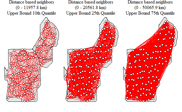
Neighborhood network with different upper bound values
As you can see the number of links between locations increases as the upper bound is expanded thereby increasing the average number of links within the network. How would this potentially influence the detection of clusters within the data set. Remember the last Hot-Spot blog post? Well lets run through the code, below is using the 10th quantile as the upper bound as an example.
# Convert nearest neighbor to a list
nb_lw<-nb2listw(nb.q10)

# local G
local_g<-localG(p12.shp.wca$TPSDF,nb_lw)

# convert to matrix
local_g.ma=as.matrix(local_g)

# column-bind the local_g data
p12.shp.wca<-cbind(p12.shp.wca,local_g.ma)

# change the names of the new column
names(p12.shp.wca)[ncol(p12.shp.wca)]="localg.Q10"

# determine p-value of z-score
p12.shp.wca$pval.q10<- 2*pnorm(-abs(p12.shp.wca$localg.Q10))

# See if any site is a "Hot-Spot"
subset(p12.shp.wca@data,localg.Q10>0&pval.q10<0.05)$STA_ID
## [1] "M009" "M011" "M012" "M014" "M015" "M024" "M025" "M027" "M028" "M029"
## [11] "M032" "M033" "M034" "M260" "M261" "M262" "M274" "M276" "M278" "M280"
## [21] "M282"Looks like a couple of sites are considered Hot-Spots. Now do that same thing for nb.q25 and nb.q75 and this is what you get.
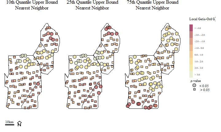
Soil total phosphorus hot-spots identified using the Getis-Ord \(G_{i}^{*}\) spatial statistic based on different nearest neighbor bands.
Hot-Spots are identified with \(G_{i}^{*}\) > 0 and associated with significant \(\rho\) values (in this cast our \(\alpha\) is 0.05). Alternatively “Cold-Spots”, or areas associated with clustering of relatively low values are identified with \(G_{i}^{*}\) < 0 (and significant \(\rho\) values). Across the three different distance bands, you can see a potential shift in Hot-Spots and the occurrence (and shift) of Cold-Spots across the study area.
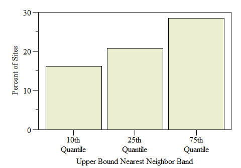
Number of sites identified as Hot-Spots across the study by Nearest Neigbhor upper bound band.
An alternative to selecting distance bands is to use a different approach such as K-function or K nearest neighbors. K-function summarizes the distance between points for all distances (Gimond 2020). This method can also be sensitive to distance bands but less so than above. In k-function nearest neighbor using knearneigh(), the function will eventually give a warning letting you know but will still compute the values anyways.
Warning messages:
1: In knearneigh(p12.shp.wca, k = 45) :
  k greater than one-third of the number of data points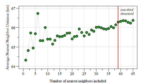
The affect of the number of nearest neighbors on average nearest neighbor distance.
Based on the plot above, a k=6 seems to be conservative enough. As suggested in the last blog post this could be done by…
# Convert nearest neighbor to a list
nb_lw<-nb2listw(k1)

# local G
local_g<-localG(p12.shp.wca$TPSDF,nb_lw)

# convert to matrix
local_g.ma=as.matrix(local_g)

# column-bind the local_g data
p12.shp.wca<-cbind(p12.shp.wca,local_g.ma)

# change the names of the new column
names(p12.shp.wca)[ncol(p12.shp.wca)]="localg.k"

# determine p-value of z-score
p12.shp.wca$pval.k<- 2*pnorm(-abs(p12.shp.wca$localg.k))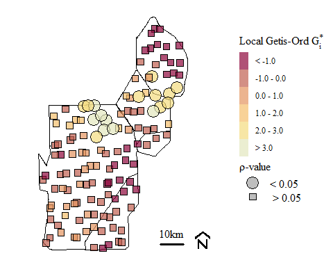
Soil total phosphorus hot-spots identified using the Getis-Ord \(G_{i}^{*}\) spatial statistic with k-function nearest neighbor spatial weighting.
using K-function nearest neighbor we have the occurrence of Hot-Spots in the general area of the other evaluations presented above. As suggested in the original Hot-Spot blog, the selection of spatial weights is important and the test is sensitive to the weights assigned.
The next post will cover how spatial aggregation can play a role in Hot-Spot detection. Until then I’ll leave you with this quote that helps put spatial statistical analysis into perspective.
“The first law of geography: Everything is related to everything else, but near things are more related than distant things.” (Tobler 1970)
Cox, D. R. 1977. “The Role of Significance Tests.” Scandinavian Journal of Statistics 4 (2): 49–63. https://www.jstor.org/stable/4615652.
Diggle, Peter J. 2006. “Spatio-Temporal Point Processes: Methods and Applications.” Monographs on Statistics and Applied Probability 107: 1–45.
Fortin, Marie-Josée, and Mark R. T. Dale. 2005. Spatial Analysis: A Guide for Ecologists. Cambridge University Press.
Gimond, Manuel. 2020. Intro to GIS and Spatial Analysis. https://mgimond.github.io/Spatial/index.html.
Tobler, W. R. 1970. “A Computer Movie Simulating Urban Growth in the Detroit Region.” Economic Geography 46 (June): 234. https://doi.org/10.2307/143141.